Note

Click here to download the full example code

Using external samples easily

emcee, arviz, and numpyro are all popular MCMC packages. ChainConsumer provides class methods to turn results from these packages into chains efficiently.

If you want to request support for another type of chain, please open a discussion with a code example, and we can add it in. The brave may even provide a PR!

import arviz as az
import emcee
import numpy as np
import numpyro
import numpyro.distributions as dist
from jax import random
from numpyro.infer import MCMC, NUTS
from scipy.stats import norm

from chainconsumer import Chain, ChainConsumer

Emcee

Let's make a dummy model here.

# Of course, your code is probably a bit more complex
def run_emcee_mcmc(n_steps, n_walkers):
    rng = np.random.default_rng(42)
    observed_data = rng.normal(loc=1, scale=1, size=100)

    def log_likelihood(theta, data):
        mu, log_sigma = theta
        return np.sum(norm.logpdf(data, mu, np.exp(log_sigma)))

    def log_prior(theta):
        mu, log_sigma = theta
        if -10 < mu < 10 and -10 < log_sigma < 10:
            return 0.0
        return -np.inf

    def log_probability(theta, data):
        lp = log_prior(theta)
        if not np.isfinite(lp):
            return -np.inf
        return lp + log_likelihood(theta, data)

    ndim = 2
    p0 = rng.uniform(low=0, high=1, size=(n_walkers, ndim))
    sampler = emcee.EnsembleSampler(n_walkers, ndim, log_probability, args=(observed_data,))
    sampler.run_mcmc(p0, n_steps, progress=False)

    return sampler


sampler = run_emcee_mcmc(8000, 16)
params = [r"$\mu$", r"$\log(\sigma)$"]
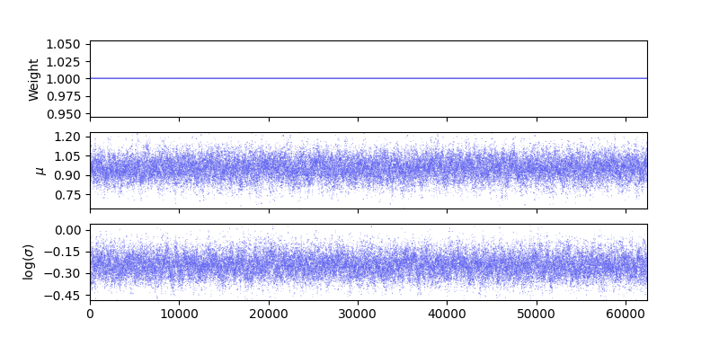
chain = Chain.from_emcee(sampler, params, "an emcee chain", discard=200, thin=2, color="indigo")
consumer = ChainConsumer().add_chain(chain)

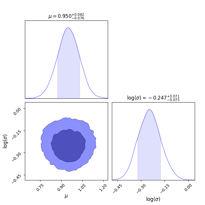
Let's plot the walks to make sure we've discard enough burn-in

fig = consumer.plotter.plot_walks()

And then show the contours themselves

fig = consumer.plotter.plot()

Numpyro

Let's start with numpyro. Again, let's make a dummy model we can sample from.

def run_numpyro_mcmc(n_steps, n_chains):
    rng = np.random.default_rng(42)
    observed_data = rng.normal(loc=0, scale=1, size=100)

    def model(data):
        # Prior
        mu = numpyro.sample("mu", dist.Normal(0, 10))
        sigma = numpyro.sample("sigma", dist.HalfNormal(10))

        # Likelihood
        with numpyro.plate("data", size=len(data)):
            numpyro.sample("obs", dist.Normal(mu, sigma), obs=data)  # type: ignore

    # Running MCMC
    kernel = NUTS(model)
    mcmc = MCMC(kernel, num_warmup=500, num_samples=n_steps, num_chains=n_chains, progress_bar=False)
    rng_key = random.PRNGKey(0)
    mcmc.run(rng_key, data=observed_data)

    return mcmc


mcmc = run_numpyro_mcmc(8000, 1)
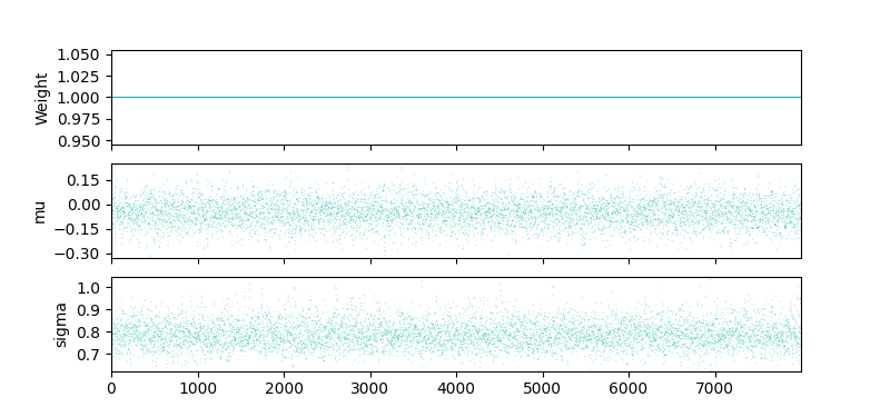
chain = Chain.from_numpyro(mcmc, "numpyro chain", color="teal")
consumer = ChainConsumer().add_chain(chain)

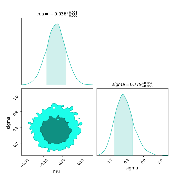
Let's plot the walks to make sure we've discard enough burn-in

fig = consumer.plotter.plot_walks()

And then show the contours themselves

fig = consumer.plotter.plot()

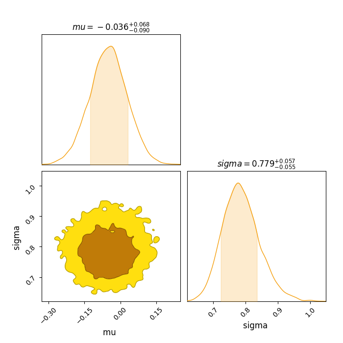
Arviz

To simplify the process, we're going to make our arviz sample from the numpyro one.

arviz_id = az.from_numpyro(mcmc)
chain = Chain.from_arviz(arviz_id, "arviz chain", color="amber")
fig = ChainConsumer().add_chain(chain).plotter.plot()

Total running time of the script: ( 0 minutes 22.316 seconds)

Download Python source code: plot_5_emcee_arviz_numpyro.py

Download Jupyter notebook: plot_5_emcee_arviz_numpyro.ipynb

Gallery generated by mkdocs-gallery