Note

Click here to download the full example code

Miscellanous Visual Options¶

Rather than having one example for each option, let's condense things.

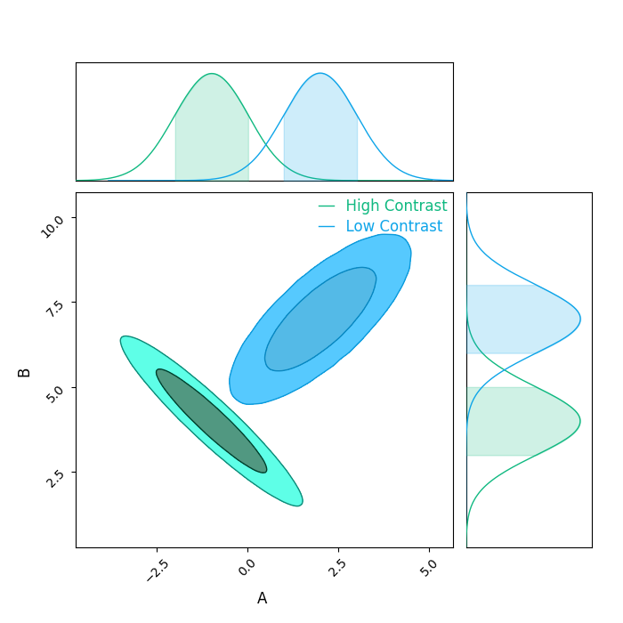
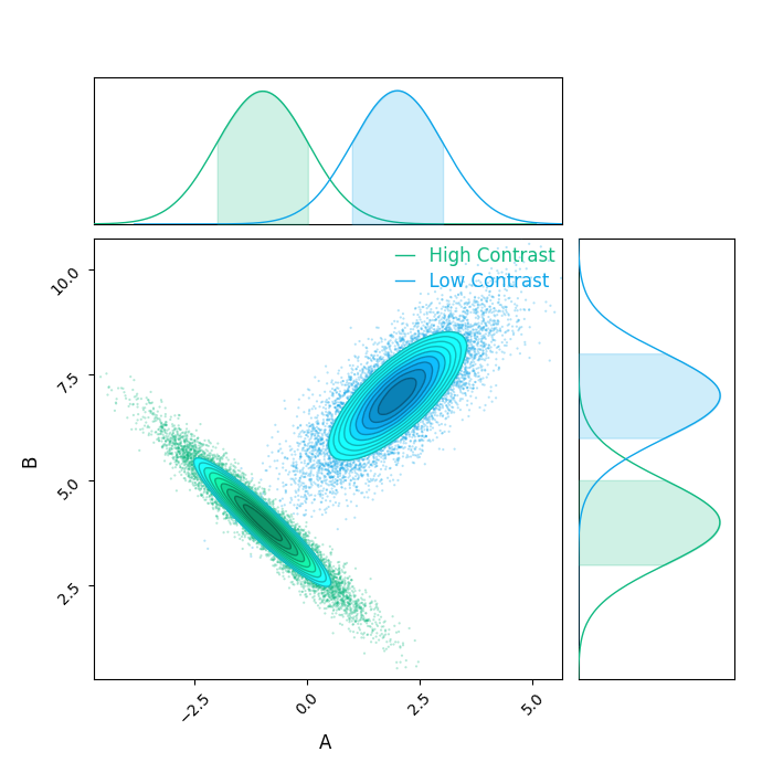
Shade Gradient¶

Pretty simple - it controls how much visual difference there is in your contours.

import numpy as np

from chainconsumer import Chain, ChainConfig, ChainConsumer, PlotConfig, make_sample

df1 = make_sample(num_dimensions=2, seed=3) - 1
df2 = make_sample(num_dimensions=2, seed=1) + 2

c = ChainConsumer()
c.add_chain(Chain(samples=df1, name="High Contrast", color="emerald", shade_gradient=2.0))
c.add_chain(Chain(samples=df2, name="Low Contrast", color="sky", shade_gradient=0.2))

c.set_plot_config(PlotConfig(flip=True))
fig = c.plotter.plot()

plot 4 misc chain visuals

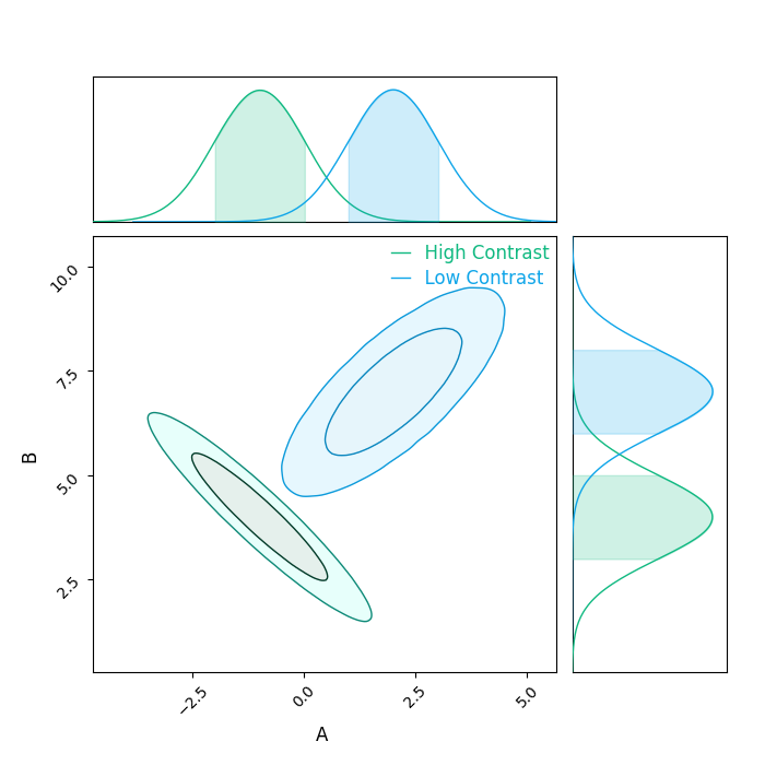
Shade Alpha¶

Controls how opaque the contours are. Like everything else, you can specify this when making the chain, or apply a single override to everything like so.

c.set_override(ChainConfig(shade_alpha=0.1))
fig = c.plotter.plot()

plot 4 misc chain visuals

Contour Labels¶

Add labels to contours. I used to have this configurable to be either sigma levels or percentages, but there was confusion over the 1D vs 2D sigma levels, in that $1\sigma$ in a 2D gaussian is not 68% of the volume. So now we just do percentages.

c.set_override(ChainConfig(show_contour_labels=True))
fig = c.plotter.plot()

plot 4 misc chain visuals

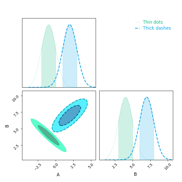
Linestyles and widths¶

Fairly simple to do. To show different ones, I'll remake the chains, rather than having a single override. Note you could try something like chain.line_width = 5, but this is a sneaky override, and it won't be registered in the internal "You set this attribute and didn't use the default when you made the chain, so don't screw with it."

Nothing does screw with line width, or similar, but it's a good habit.

c2 = ChainConsumer()
c2.add_chain(Chain(samples=df1, name="Thin dots", color="emerald", linestyle=":", linewidth=0.5))
c2.add_chain(Chain(samples=df2, name="Thick dashes", color="sky", linestyle="--", linewidth=2.0))
fig = c2.plotter.plot()

plot 4 misc chain visuals

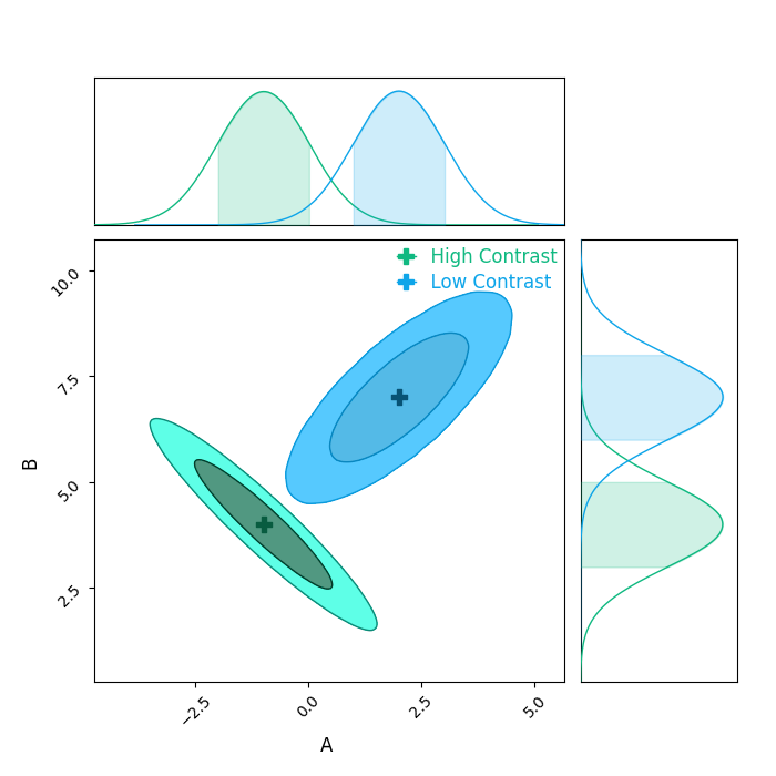
Marker styles and sizes¶

Provided you have a posterior column, you can plot the maximum probability point.

c.set_override(ChainConfig(plot_point=True, marker_style="P", marker_size=100))
fig = c.plotter.plot()

plot 4 misc chain visuals

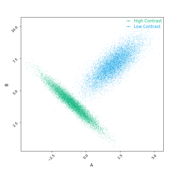
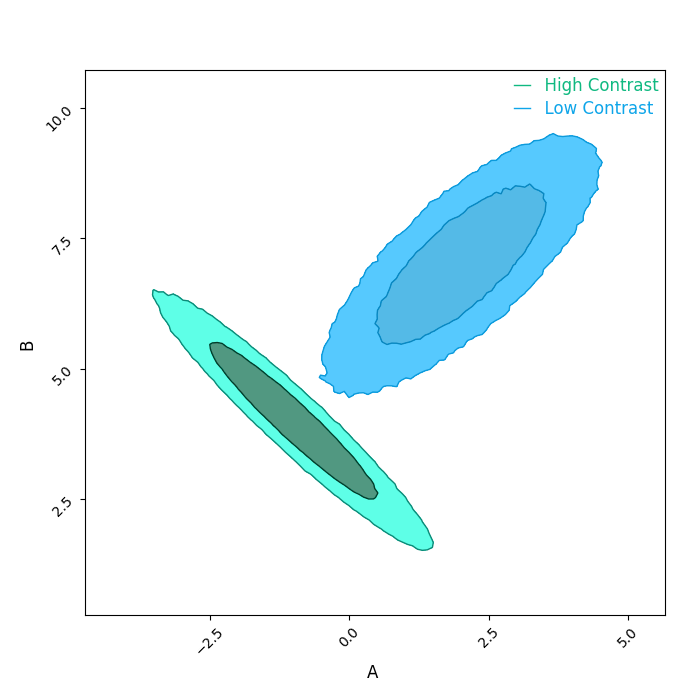
Cloud and Sigma Levels¶

Choose custom sigma levels and display point cloud.

c.set_override(
    ChainConfig(
        shade_alpha=1.0,
        sigmas=np.linspace(0, 1, 10).tolist(),
        shade_gradient=1.0,
        plot_cloud=True,
    )
)
fig = c.plotter.plot()

plot 4 misc chain visuals

Of course, you don't have to change both at once. Here's just a cloud. And also note that contours include the 2D marginalised distributions, hence why I am hising the histograms here (as they'll be empty).

c.set_override(ChainConfig(plot_cloud=True, plot_contour=False))
c.set_plot_config(PlotConfig(plot_hists=False))
fig = c.plotter.plot()

plot 4 misc chain visuals

Smoothing (or not)¶

The histograms behind the scene in ChainConsumer are smoothed. But you can turn this off. The higher the smoothing vaule, the more subidivisions of your bins there will be.

c.set_override(ChainConfig(smooth=0))
fig = c.plotter.plot()

plot 4 misc chain visuals

But changing the smoothing doesn't change the number of bins. That's separate.

c.set_override(ChainConfig(smooth=0, bins=10))
fig = c.plotter.plot()

plot 4 misc chain visuals

It's beautiful. And it's hard to find a nice balance.

c.set_override(ChainConfig(smooth=0, bins=100))
fig = c.plotter.plot()

plot 4 misc chain visuals

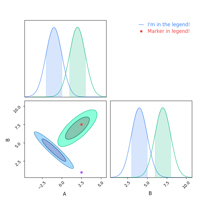
Controlling the legend¶

Sometimes we have a bunch of things we want to show, whether they are chains, markers, truth values, or something else. By default, ChainConsumer will try to show everything, but you specifically tell it to hide items on the legend.

c = ChainConsumer()
c.add_chain(Chain(samples=df1, name="I'm in the legend!"))
c.add_chain(Chain(samples=df2, name="I'm not!", show_label_in_legend=False))
c.add_marker(location={"A": 2.5, "B": 7.5}, marker_size=100, name="Marker in legend!")
c.add_marker(location={"A": 2.5, "B": 1}, marker_size=100, name="Marker not in legend", show_label_in_legend=False)
fig = c.plotter.plot()

plot 4 misc chain visuals

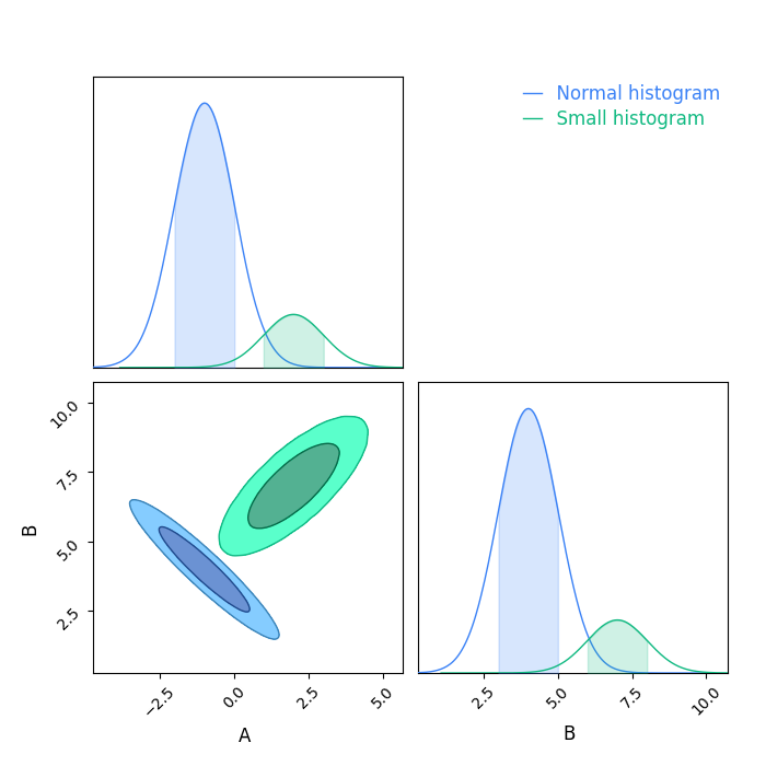
Changing the height of the histogram¶

For very niche reasons, you may want to change the defaults so that the marginalised histograms on the diagonal are not normalised to unit area. You can set the histogram_relative_height value to change this, such that a value of 0.5 would mean "Make the histogram half as tall" and thus result in a normalised area of 0.5 instead of 1.0.

c = ChainConsumer()
c.add_chain(Chain(samples=df1, name="Normal histogram"))
c.add_chain(Chain(samples=df2, name="Small histogram", histogram_relative_height=0.2))
c.set_plot_config(PlotConfig(flip=False))
fig = c.plotter.plot()